HOW-TO Visualize observational pointings with ObsViewer (OLD)
ObsViewer can query the database for RawScienceFrames or ReducedScienceFrames for a given rectangular region of the sky, wavelength range and range in exposure time. It can output the results in a figure and ascii files.
NOTE1: EXPERIMENTAL VERSION. Bug reports and other feedback welcome: Gijs Verdoes Kleijn (verdoes@astro.rug.nl)
NOTE2: ONLY WFI OBSERVATIONAL POINTINGS ARE QUERIED.
Example 1 of use at the awe-prompt
1 2 3 4 5 6 7 8 | awe> from astro.experimental.ObsViewer import ObsViewer
awe> o = ObsViewer()
awe> o.query_database(rastart=174, raend=178, decstart=-5, decend=-5,
central_lambdastart=4000.0, central_lambdaend=5000.0,
expomin=0.0, expomax=200.0,raw='yes')
awe> o.preview(newplot=1, plotcolor='b', plotsize=20)
awe> o.plot(plotfov=1, fillfov=1, newplot=1, plotcolor='b',
plotsize=20, sec_per_dot=1.0)
|
The command lines have the following effects:
IMPORTS MODULE INTO AWE ENVIRONMENT.
MAKES A CLASS INSTANTIATION.
- QUERIES THE DATABASE.Input parameters:
- rastart/end: (degrees) start and end right ascension of rectangular region in the sky.
- decstart/end: (degrees) start and end declination of rectangular region in the sky.
- central_lambdastart/end: (Angstrom) start and end of wavelength region in which the central wavelength of the exposure filter has to be.
- expomin/max: (sec) minimum/maximum exposure time for exposure.
- raw: query for raw images (raw=’yes’) or reduced images (raw=’no’).
Result:a query which can be used by o.preview and o.plot. - PLOTS AND SAVES A FIGURE CONTAINING ONLY THE POINTING CENTERS OF THE QUERY RESULTS.Input parameters:
- newplot: make a new plot (newplot=1) or overplot on an existing one (newplot=0)?
- plotcolor: color of plotting symbol: color=’r’ means red, and b:blue, g:green, c:cyan, m:magenta, y:yellow, k:black, w:white.
- plotsize: size of the plotting symbol to plot.
Output:a figure (png format) named ObsViewer_ra_\(<\)rastart\(>\)_\(<\)raend\(>\)_dec_\(<\)decstart\(>\)_\(<\)decend\(>\)-_lambda_:math:<lambdastart\(>\)_\(<\)lambdaend\(>\)_expo_\(<\)expomin\(>\)_\(<\)expomax\(>\)_preview.png (see Figure [f:preview]).NOTE: the tool buttons on the bottom of the graphical display window can be used to zoom in on parts of the figure.
- PLOTS AND SAVES A FIGURE VISUALIZING THE QUERY RESULT AND WRITES AN OUTPUT FILE WITH THE RESULTS.Input parameters:
- plotfov: plot the field of view (FOV) around the pointing centers (0=no, 1=yes)?
- fillfov: fill the FOV with random poisson points (to emphasize overlapping exposures) (0=no, 1=yes)?
- sec_per_dot: the number seconds exposure time per dot plot by fillfov. For example, sec_per_dot=10.0 plots a dot for each ten seconds of exposure time.
- plotcolor: color of plotting symbol: color=ŕ’ means red, and b:blue, g:green, c:cyan, m:magenta, y:yellow, k:black, w:white.
- plotsize: size of the plotting symbol to plot.
Outputs:A graphical display window with the result.A figure (png format) named ObsViewer_ra_\(<\)rastart\(>\)_\(<\)raend\(>\)_dec_\(<\)decstart\(>\)_\(<\)decend\(>\)-_lambda_:math:<lambdastart\(>\)_\(<\)lambdaend\(>\)_expo_\(<\)expomin\(>\)_\(<\)expomax\(>\).png (see Figure [f:plot]). A text file (ascii format) named ObsViewer_ra_\(<\)rastart\(>\)_\(<\)raend\(>\)_dec_\(<\)decstart\(>\)_\(<\)decend\(>\)-_lambda_:math:<lambdastart\(>\)_\(<\)lambdaend\(>\)_expo_\(<\)expomin\(>\)_\(<\)expomax\(>\).txt.NOTE: the tool buttons on the bottom of the graphical display window can be used to zoom in on parts of the figure.
Example 2
1 2 3 4 5 6 7 | awe> from astro.experimental.ObsViewer import ObsViewer
awe> o = ObsViewer()
awe> o.query_database(rastart=170, raend=180, decstart=-20, decend=-20, central_lambdastart=4000.0, central_lambdaend=5000.0, expomin=0.0, expomax=200.0, raw='yes')
awe> o.plot(plotfov=1, fillfov=1, newplot=1, plotcolor='b', plotsize=20, sec_per_dot=1.0)
awe> o.query_database(rastart=170, raend=180, decstart=-20, decend=-20, central_lambdastart=5000.0, central_lambdaend=6000.0, expomin=0.0, expomax=200.0, raw='yes')
awe> o.plot(plotfov=1, fillfov=1, newplot=0, plotcolor='g', plotsize=20, sec_per_dot=1.0)
|
Command lines have the following effects:
-.4: similar to steps in example 1.
Now the query is made for frames with a central_lambda different from step 3
The result from the query in step 5 is overplotted in green on the existing plot from step 4 (see Figure 3).
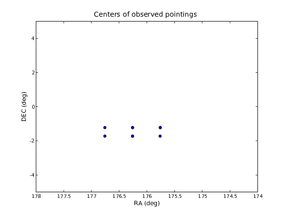
Figure 1: Example output figure from awe> o.preview(). The circles
indicate the centers of the pointings
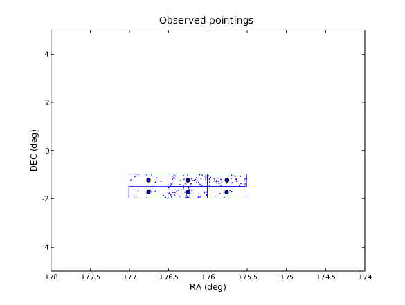
Figure 2: Example output figure from awe> o.plot(plotfov=1,fillfov=1).
The rectangles represent the FOV of the exposure to scale. The random dots
(by setting fillfov=1) reflect the exposure time as explained in example 1.
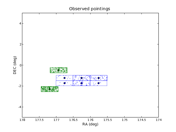
Figure 3: Example output figure from two queries as in example 2. The rectangles represent the FOV of the exposure to scale. The random dots (by setting fillfov=1) reflect the exposure time as explained in example 1.